01 Introduction
When an imagined trajectory returns to a previously visited state, a world model should render the same place. We call this requirement spatial persistence. World models predict observations under actions, allowing agents to anticipate the consequences of their behavior without further interaction with the environment [1, 2]. In many recurrent state-space models [2, 3], transformers [4] and diffusion-based models [5], scene layout, appearance and agent motion are carried together in an evolving predictive representation. Over a long rollout, accumulated errors can change the scene that this representation describes. Individual frames may remain plausible while a familiar corridor looks different when the agent returns.
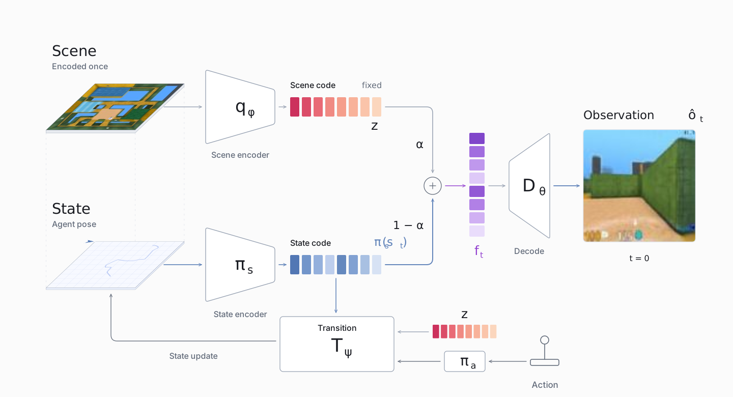
Space-Aware World Models (SWM) are generative models that separate persistent scene memory from agent dynamics (Figure 1). A scene code is encoded from a top-down map or sampled from the prior to generate a new environment, then held fixed throughout the rollout. An action-conditioned transition model evolves the explicit agent state , and a renderer produces observations from . Training uses map-like observations and low-dimensional state supervision, with scene layouts assumed static within each episode. We study this setting with compact models trained on a single workstation.
02 Space-Aware World Model
Let denote a top-down map, the agent state and the action. With state and action encoders and , SWM defines three components:
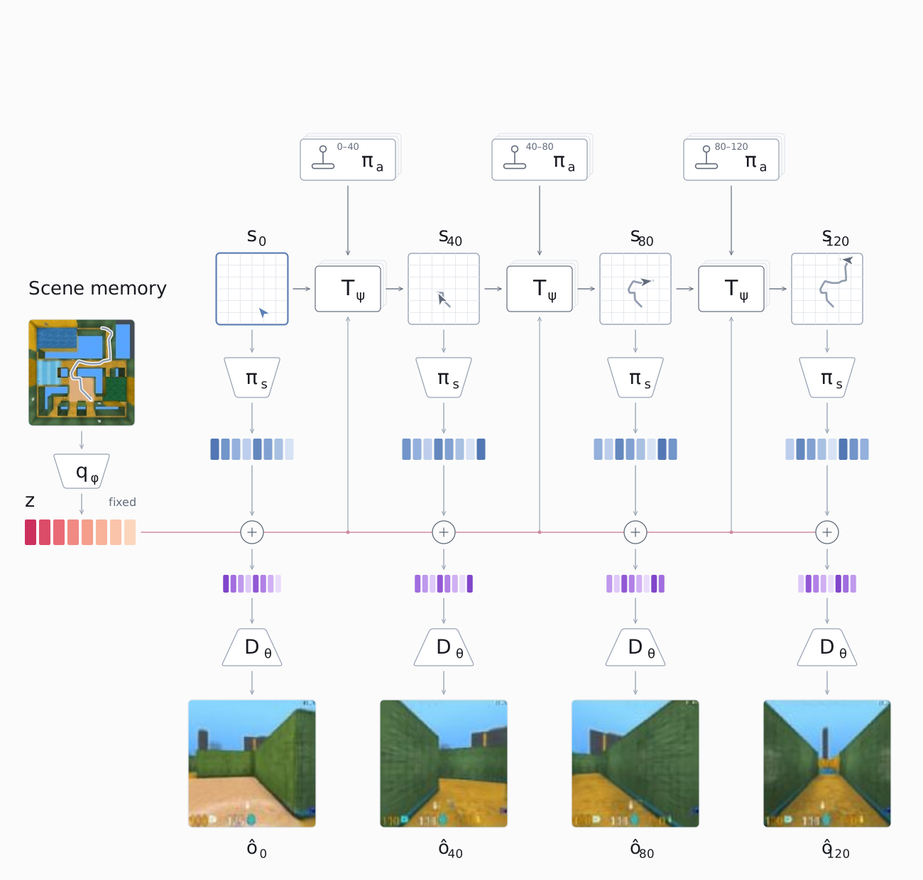
A rollout starts with a scene code, obtained by encoding a map once or sampling from the prior to generate a new environment. The model then alternates between rendering an observation and updating the agent state (Figure 2). The scene code remains fixed throughout. Autoregressive prediction acts only on the explicit agent state, such as position and heading.
2.1 Scene Encoder
The scene encoder is a variational autoencoder [6] that maps a top-down image to a compact scene code. The shared encoder maps held-out layouts into the same latent space without per-scene optimization, unlike the scene-specific fitting used by methods such as NeRF [7]. Its prior also allows new scene codes to be sampled. Figure 3 illustrates the scene-code manifold through a projection onto the first two principal components.
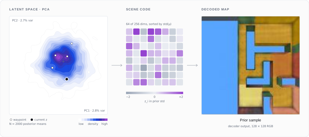
The scene prior lets SWM generate new environments without an input map: a sampled code can be decoded into a map and used directly by the observation and transition models (Figure 4).
2.2 Observation Model
The observation model is a deterministic renderer conditioned on the scene code and current state. A Fourier feature transform [8] and a linear projection map the state to , the same dimensionality as the scene code. The two pathways meet through bounded additive fusion,
which the decoder maps to the observation . The mixing weight is a learned scalar shared across scenes within each domain. The bound keeps both fusion weights nonzero, discouraging reliance on state alone. Training combines a pixel reconstruction loss with a perceptual loss [9].
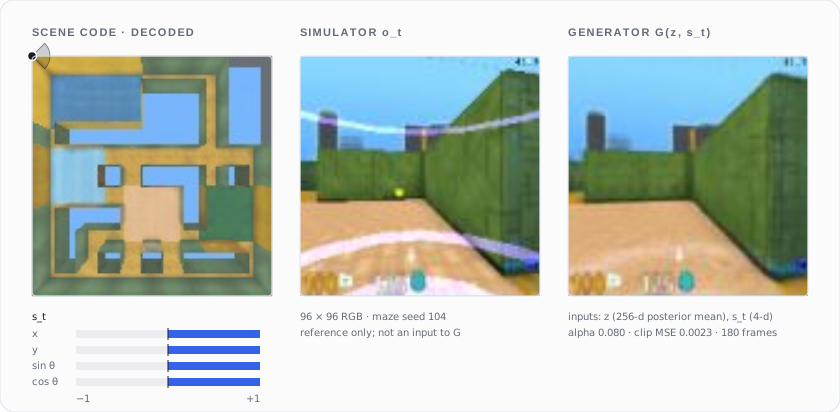
For a fixed scene code, the same state always produces the same rendered observation. The learned dynamics can still accumulate state drift. Before decoding, error separates into a constant scene term and a time-varying state term . This is a decomposition in fusion space, not in image pixels. Rendering at the ground-truth state removes the second term and defines the SWM-oracle variant in Section 5.4. Figure 5 shows the renderer along a recorded trajectory, using only the scene code and the agent’s pose, represented here by .
03 Transition Model and Wall Contacts
The transition model uses the scene code as context to predict action-conditioned state increments:
The explicit state describes the agent, while the scene code provides the geometric context for . The same state–action pair can therefore produce different increments in an open region and near an obstacle. Predicting increments is a natural fit for these domains, where consecutive motions are small relative to the environment. It also makes rollout error interpretable as gradual mislocalization in physical state space.
Figure 6 probes whether the transition model uses this scene information. Starting from the first recorded state of an episode held out from transition-model training, we run under the recorded actions without correcting its predictions. With the episode’s own scene code, the predicted trajectory follows the recording, including stops at wall contacts. Replacing only the scene code with that of a different map causes the prediction to diverge at the first wall contact.
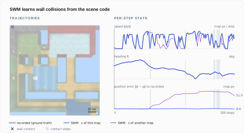
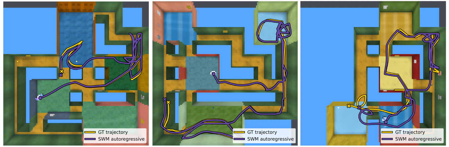
The transition model learns motion and wall contacts from recorded transitions, without explicit collision checks or map lookups (Section 04). The longer held-out trajectories in Figure 7 follow local map structure and obstacle-induced turns while gradually accumulating state drift.
04 Data Collection with Fast Sweeping
For the DeepMind Lab (DMLab) [10] navigation experiments, we collect training rollouts with a map-guided procedure that requires no pretrained exploration policy. A random policy can remain in a small part of a maze and provide limited coverage. To collect longer traversals, we guide the agent with the episode’s top-down map.
We first segment each map into a binary occupancy grid, separating free space from walls. After sampling a waypoint in free space, we compute the geodesic travel time from each free cell to by solving the eikonal equation
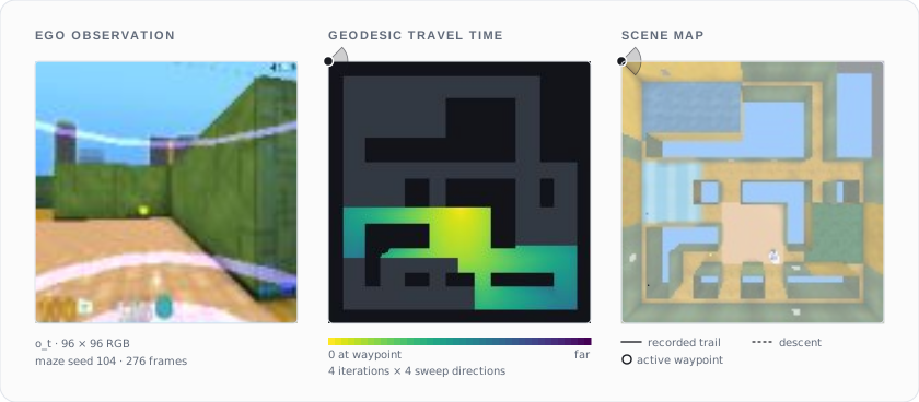
with walls excluded from the domain. The fast sweeping method [11, 12] solves this equation using Gauss–Seidel upwind updates in four alternating sweep orders. Each cell is updated from the smallest neighboring values along the two grid axes. Figure 8 illustrates how successive sweeps propagate travel times around obstacles.
The negative gradient points along a shortest path through free space to the waypoint, bending around walls. We convert this direction into environment actions using the agent’s current pose. Small stochastic perturbations encourage varied trajectories and broader state-space coverage. When the agent reaches the waypoint, we sample a new one and recompute the field.
These trajectories cover long traversals and wall contacts, providing examples of how scene geometry constrains motion (Figure 6).
We train the three modules sequentially: the scene encoder on maps, the observation model on tuples with precomputed scene codes, and the transition model on action-conditioned state sequences with as context.
05 Experiments
5.1 Experimental Setup
We evaluate on two procedurally generated domains with held-out layouts. DMLab tests revisitation and return-to-origin consistency in first-person 3D navigation. CarRacing [13] tests whether generated observations preserve the track information used by a controller. Training uses 2 × 10⁴ episodes, roughly 107 frames, with one top-down image per episode. We compare SWM with compact implementations of four latent-dynamics families: an MDN-RNN world model [1], an IRIS-style transformer [4], DreamerV3 [3] and LeWM [14]. All systems use the same rollout data and action sequences, with workstation-scale training budgets. SWM additionally receives a top-down map and state supervision. These cross-family comparisons therefore evaluate the complete structured approach; they do not isolate the effect of factorization under equal input information.
5.2 DMLab: First-Person Navigation
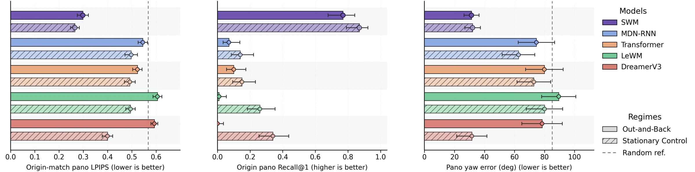
We evaluate long imagined rollouts on held-out layouts. State-match LPIPS [9] measures perceptual agreement between generated and real observations at matched physical states, including revisits separated by long temporal gaps. The return-to-origin benchmark tests place identity with full panoramas captured at the start and after an out-and-back excursion. Origin-match LPIPS compares each returned view with the real start view at the same yaw. Recall@1 tests whether the returned panorama retrieves its own episode from a gallery of real start panoramas. Yaw error measures the angular offset of the best circular match.
| Metric | MDN-RNN | Transformer | DreamerV3 | LeWM | SWM | Rel. Imp. (%) |
|---|---|---|---|---|---|---|
| State-match LPIPS ↓ | 0.208± 0.115 | 0.168± 0.140 | 0.269± 0.185 | 0.407± 0.142 | 0.033± 0.061 | +80% |
| Origin-match pano LPIPS ↓ | 0.545± 0.098 | 0.523± 0.098 | 0.593± 0.070 | 0.613± 0.094 | 0.298± 0.117 | +43% |
| Origin pano Recall@1 ↑ | 0.070± 0.255 | 0.100± 0.300 | 0.000± 0.000 | 0.010± 0.099 | 0.770± 0.421 | +670% |
| Pano yaw error (deg) ↓ | 74.6± 61.5 | 79.3± 63.6 | 78.4± 68.4 | 89.5± 57.7 | 31.4± 25.4 | +57% |
| PRDC Density ↑ | 0.0659 | 0.1462 | 0.0057 | 0.0253 | 0.3710 | +154% |
| PRDC Coverage ↑ | 0.1024 | 0.2078 | 0.0086 | 0.0402 | 0.5288 | +154% |
| ECS Inlier Ratio ↑ | 0.2176 | 0.2396 | 0.0521 | 0.2878 | 0.3507 | +22% |
SWM better preserves local appearance and place identity on revisits, with closer perceptual matches, more reliable panorama retrieval and lower yaw error than the latent-dynamics baselines (Table 1). Higher PRDC density and coverage [15] also suggest that this consistency is not achieved by collapsing to a small set of plausible frames. Geometric agreement improves as well: a larger fraction of SIFT correspondences [16] agrees with the known camera motion, as measured by the ECS inlier ratio using epipolar agreement [17].
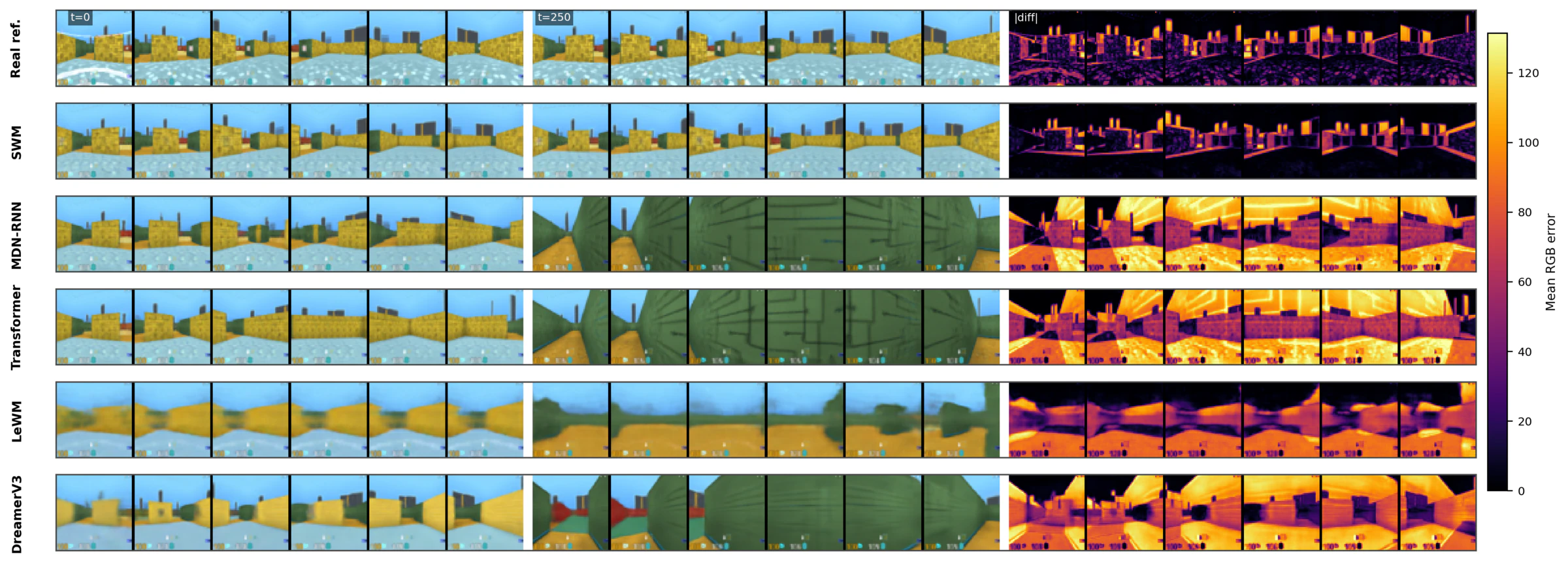
Figure 9 compares the out-and-back excursion with stationary control, where the model receives no-op actions while the ground-truth pose remains fixed. Both regimes use the same panorama protocol. SWM remains stable under stationary control and degrades moderately after the excursion, consistent with a retained scene code and accumulated transition drift. Several baselines perform poorly even under stationary control, suggesting that path integration alone does not explain their errors: scene or pose information can drift within an evolving predictive state. Figure 10 shows the return panorama of one held-out episode; Figure 11 compares imagined rollouts under the same actions.
5.3 CarRacing: Continuous Control
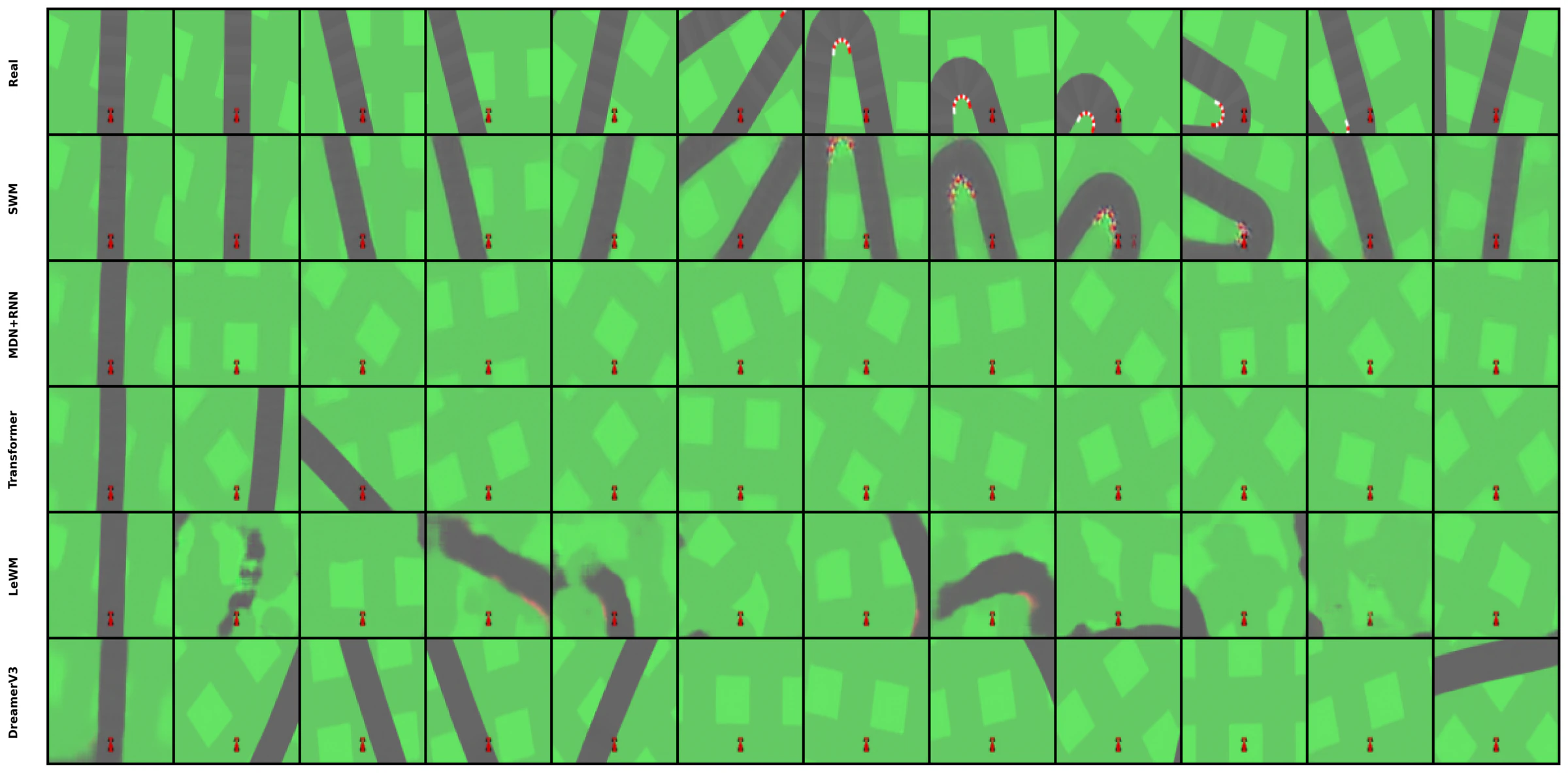
In CarRacing, we evaluate generated observations with a frozen pixel-based controller that was never trained on generated frames. SWM’s generated views lead to action distributions closer to those from real rollouts and better preserve the controller’s steering decisions on paired frames than the latent-dynamics baselines (Table 2). These results show that the observations retain information used by a fixed controller; they do not evaluate policy learning inside SWM.
| Dream action statistics | Matched-frame agreement | |||||
|---|---|---|---|---|---|---|
| Model | Action W1 ↓ | Action JS ↓ | Coupling err. ↓ | Action err. ↓ | Steer sign ↑ | Steer corr. ↑ |
| SWM | 0.023± 0.034 | 0.002± 0.001 | 0.007 | 0.655± 0.469 | 0.958 | 0.891 |
| LeWM | 0.077± 0.096 | 0.019± 0.020 | 0.209 | 1.367± 0.908 | 0.640 | 0.127 |
| Transformer | 0.085± 0.077 | 0.018± 0.014 | 0.093 | 1.423± 0.704 | 0.755 | 0.091 |
| DreamerV3 | 0.063± 0.054 | 0.014± 0.012 | 0.097 | 1.446± 0.998 | 0.627 | 0.147 |
| MDN-RNN | 0.104± 0.098 | 0.023± 0.018 | 0.205 | 1.467± 0.789 | 0.624 | -0.025 |
5.4 Horizon Diagnostics
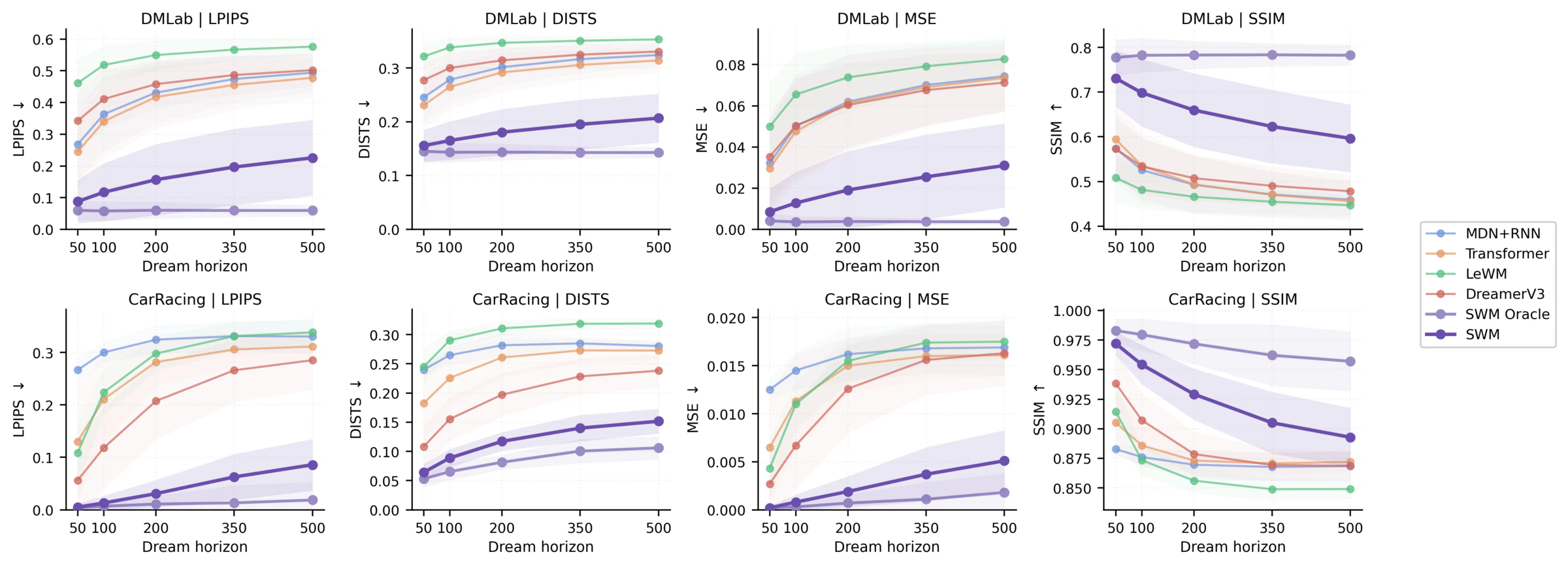
Figure 13 shows how frame fidelity changes with rollout length in both domains. The SWM-oracle variant uses the same scene code and renderer as SWM, but renders at the ground-truth state instead of the predicted state. This removes accumulated transition drift while retaining scene encoding and rendering errors. SWM degrades more slowly than the baselines, and the flatter oracle curves identify state-transition drift as a major source of its remaining long-horizon error.
5.5 Matched Scene and State Information
Cross-family comparisons cannot isolate the effect of factorization from the additional scene and state information available to SWM. To test the representation directly, we compare it with an entangled-latent control given the same pretrained scene code, initial state, actions, state supervision, data, renderer, sequence length and training budget, with comparable recurrent capacity. The control folds scene and state into one evolving code instead of keeping scene memory fixed. Both methods have similar cumulative LPIPS at shorter horizons, with the control slightly ahead at an intermediate horizon. SWM retains lower error over longer rollouts and higher panorama retrieval accuracy under repeated no-op updates (Table 3). The control’s loss of place identity without physical motion supports the role of a persistent, separately accessible scene representation.
| Metric | SWM | Entangled-latent control |
|---|---|---|
| H = 10 cumulative LPIPS ↓ | 0.0861 | 0.0882± 0.0003 |
| H = 200 cumulative LPIPS ↓ | 0.1631 | 0.1581± 0.0014 |
| H = 500 cumulative LPIPS ↓ | 0.2256 | 0.3341± 0.0026 |
| Out-and-back Recall@1 ↑ | 0.770 | 0.260± 0.050 |
| Stationary origin-match LPIPS ↓ | 0.2615 | 0.5408± 0.0105 |
| Stationary Recall@1 ↑ | 0.890 | 0.053± 0.015 |
06 Inference Speed
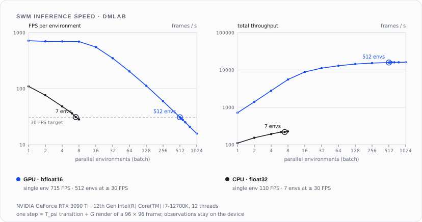
Each rollout step requires one transition of the low-dimensional state and one rendered frame. The scene code is initialized once, from a map or the prior, so the per-step cost does not grow with the rollout history. Figure 14 shows how throughput changes with the number of parallel environments. GPU batching supports many simultaneous rollouts while maintaining real-time performance per environment. The CPU also supports real-time rollouts at smaller parallel batch sizes.
07 Limitations
The quantitative evaluations use top-down maps and explicit state supervision; prior-sampled rollouts illustrate scene generation qualitatively. The cross-family baselines receive observations and actions, so those comparisons combine the effects of structured information and model design. They do not establish an advantage for generic video prediction, unknown-state settings, changing layouts or learning without map-like supervision.
A fixed scene code does not eliminate autoregressive error. The oracle diagnostics identify state-transition drift as a source of the remaining long-horizon degradation. The current formulation also assumes a compact scene code, static geometry within each episode and a single agent with a low-dimensional state. Open directions include inferring scene codes from partial observations, extending scene memory to larger or unbounded environments, modeling dynamic scenes and multiple agents, and learning policies directly within SWM rollouts.
References
- Recurrent World Models Facilitate Policy Evolution. Advances in Neural Information Processing Systems (NeurIPS), 2018.
- Dream to Control: Learning Behaviors by Latent Imagination. International Conference on Learning Representations (ICLR), 2020.
- Mastering Diverse Control Tasks through World Models. Nature, 2025.
- Transformers are Sample-Efficient World Models. International Conference on Learning Representations (ICLR), 2023.
- Diffusion for World Modeling: Visual Details Matter in Atari. Advances in Neural Information Processing Systems (NeurIPS), 2024.
- Auto-Encoding Variational Bayes. International Conference on Learning Representations (ICLR), 2014.
- NeRF: Representing Scenes as Neural Radiance Fields for View Synthesis. Computer Vision – ECCV 2020, 2020.
- Fourier features let networks learn high frequency functions in low dimensional domains. Advances in Neural Information Processing Systems (NeurIPS), 2020.
- The Unreasonable Effectiveness of Deep Features as a Perceptual Metric. Proceedings of the IEEE Conference on Computer Vision and Pattern Recognition (CVPR), 2018.
- DeepMind Lab. arXiv preprint arXiv:1612.03801, 2016.
- A fast sweeping method for eikonal equations. Mathematics of Computation, 2005.
- Level set methods and fast marching methods. 1999.
- Gymnasium: A standard interface for reinforcement learning environments. arXiv preprint arXiv:2407.17032, 2024.
- Leworldmodel: Stable end-to-end joint-embedding predictive architecture from pixels. arXiv preprint arXiv:2603.19312, 2026.
- Reliable fidelity and diversity metrics for generative models. International Conference on Machine Learning (ICML), 2020.
- Distinctive image features from scale-invariant keypoints. International Journal of Computer Vision, 2004.
- Multiple view geometry in computer vision. 2003.